Maths: From z-Scores to the Binomial Model

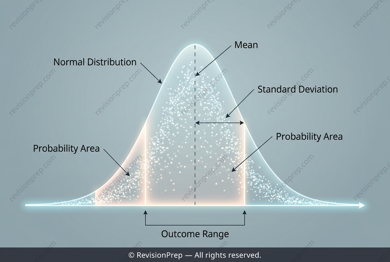
Continuous probability distributions describe outcomes that can take any value within a range, and the normal distribution is the most important example because it models natural variation around a central mean. In this context, the time for a medication to take effect is treated as a normally distributed variable, T, with a given mean and standard deviation. The key mechanism is standardisation: converting any observation into a z-score, z = (T − mean) / standard deviation, which allows probabilities to be read from the standard normal curve. This single transformation underpins all calculations of cumulative probabilities, such as finding the chance that T falls below a threshold or within an interval. The power of this concept extends beyond single observations. Once you know the probability of an event occurring for one patient, you can model how many patients out of a fixed group experience that event using a binomial distribution, B(n, p), where p is the probability from the normal calculation. Furthermore, the normal distribution’s symmetry allows you to work backwards: given a desired probability, such as 95%, you can use the inverse normal to find the symmetric interval around the mean that captures that proportion. This connects the continuous distribution to inference, showing how probabilities, counts, and confidence-style intervals all derive from the same underlying z-score logic.