Maths: Modelling a Cooling Rod with Calculus

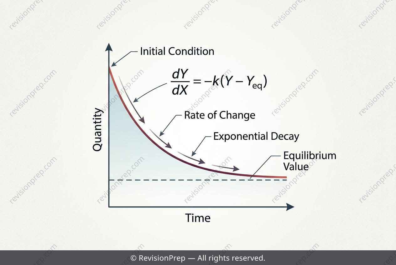
Newton’s Law of Cooling is a classic example of a first-order linear differential equation, where the rate of change of a quantity is proportional to the difference between that quantity and its surrounding environment. In this case, the temperature θ of a metal rod cools toward a fixed ambient temperature of 20°C, governed by dθ/dt = −k(θ − 20). The negative constant −k ensures that the rod cools (not heats) over time, and the solution θ = 20 + 80e^(−kt) emerges naturally from separating variables or verifying a proposed form. This model matters because exponential decay appears everywhere—from radioactive half-life to medicine dosage and even financial depreciation. The key mechanism is that the rate of change depends on how far the system is from equilibrium, not on time itself. Verifying the solution involves differentiating the proposed function and substituting back into the differential equation, while also checking the initial condition at t = 0. Then, using a given data point (like temperature after 5 minutes) allows you to solve for the decay constant k exactly, often leading to a logarithmic expression. Understanding this structure lets you predict future temperatures or find how long a process takes, making it a cornerstone of calculus applications in the IB syllabus.