Maths: Modelling Exponential Decay with Calculus

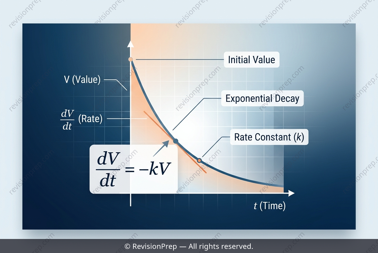
Exponential decay is one of the most elegant applications of differential equations, and it appears everywhere—from radioactive half-lives to the depreciation of assets. In this context, the rate at which a machine’s value falls is proportional to its current value, captured by the equation dV/dt = -kV. This simple relationship tells us that the more valuable the machine, the faster it loses worth, yet the proportional nature means the decline slows over time, never quite reaching zero. The solution to this differential equation is an exponential function, V = Ae^(-kt), where A is the initial value and k is the decay constant. To find A, you apply the starting condition—here, the machine begins at 50 thousand dollars. Then, using a later data point (after 3 years, the value is 40 thousand), you substitute into the model to solve for k. This involves isolating the exponential, taking a natural logarithm, and rearranging—steps that mirror the general method for any exponential decay problem. Understanding how the constant k quantifies the speed of decay, and how initial conditions anchor the curve, turns a formula into a powerful predictive tool.