Statistics and Probability

The biggest topic in IB Maths AI HL — confidence intervals, hypothesis tests, χ² and regression, made exam-ready.

Illustration of a normal distribution curve with a confidence interval shaded, a scatter plot with a regression line, and a chi-squared table

Subject

Maths AI

Curriculum

IB Diploma Programme

Grade

Topic

Statistics and Probability

Reading

9 min

Difficulty

Advanced

Quick facts

Difficulty

★★★★☆

Exam weight

~30% of AI HL (Paper 1 & 2)

Prerequisites

Algebra, basic probability, GDC statistics menu

You'll learn

Confidence intervals, hypothesis tests, χ² tests, regression

Revision time

3-4 hours

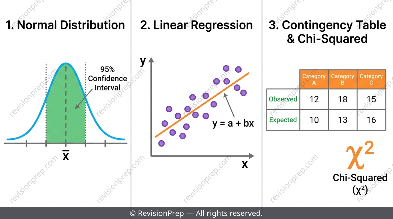
Statistics and Probability is the single largest topic in IB DP Maths AI, and at HL it's where descriptive statistics turns into genuine inference. You'll move from summarising data with the mean, standard deviation and correlation coefficient into asking harder questions: what can a sample honestly tell us about a population, and how confident can we really be? Confidence intervals, hypothesis tests (z, t, paired-t), and chi-squared tests dominate HL Paper 2 extended-response questions precisely because they combine GDC output with written interpretation — examiners want to see the setup, the test statistic, and a conclusion written in context, not just a correct number. This teaser walks through the five ideas that show up again and again: sampling and unbiased estimators, correlation vs regression, confidence intervals, hypothesis testing, and chi-squared tests — with the exact traps that lose marks.

What you’ll be able to do

✓Identify sampling methods and the bias each one risks

✓Distinguish population variance from the unbiased sample variance estimate

✓Choose between Pearson's r and Spearman's rank correlation correctly

✓Construct a confidence interval for μ using the t-distribution

✓Set up and conclude a z-test, t-test or paired t-test in context

✓Calculate expected frequencies and degrees of freedom for a χ² test

✓Avoid extrapolating beyond the range of regression data

✓Write exam-standard conclusions that state a decision AND its meaning

Sampling Methods and the Unbiased Variance

Every inference starts with a sample, so examiners test whether you know the bias each sampling method risks: simple random, systematic, stratified, quota and convenience sampling all appear as 'comment on this method' questions. On the numerical side, your GDC gives two variances — $σ_{n}^{2}$ (population) and $σ_{n - 1}^{2}$ (the unbiased sample estimate) — and mixing them up is a classic silent error.

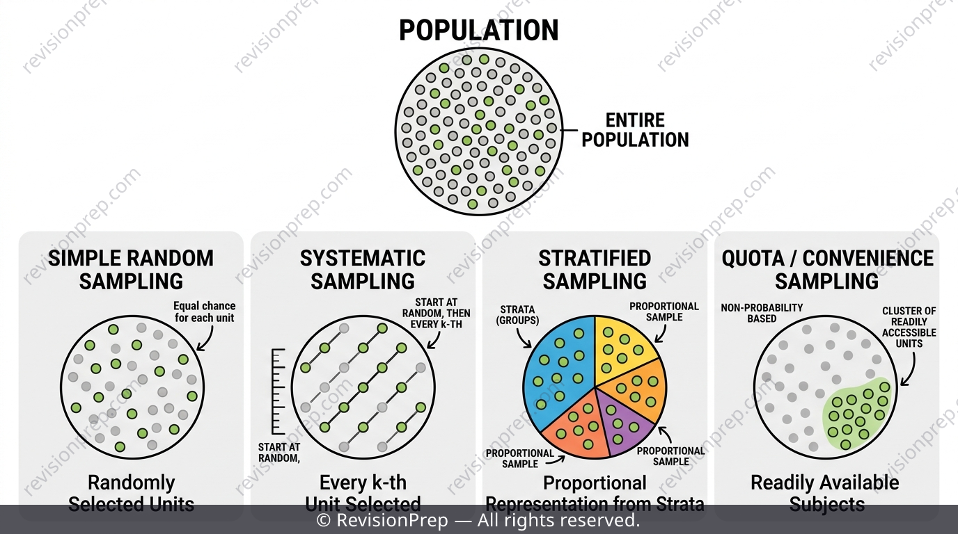
Diagram comparing simple random, systematic, stratified and quota sampling from a population circle

Sampling method	How it works	Bias risk
Simple random	Every member has equal chance of selection	Low bias, but needs a full population list
Systematic	Every k-th member after a random start	Can miss hidden patterns in the list order
Stratified	Proportional sampling from subgroups	Needs accurate subgroup sizes
Quota / Convenience	Interviewer fills quotas or samples whoever's easiest	Non-random — often badly biased

Exam tip

If a question gives you $σ_{n}$ from the GDC but asks for the 'best estimate of the population variance', switch to $s_{n - 1}^{2} = \frac{n}{n - 1} σ_{n}^{2}$ .

Common mistake

Reporting $σ_{n}$ (dividing by n) when the question actually wants the unbiased estimate $s_{n - 1}$ (dividing by n-1).

Mini summary

Know the sampling method's bias, and always check which variance button your GDC used.

Correlation, Regression and the Extrapolation Trap

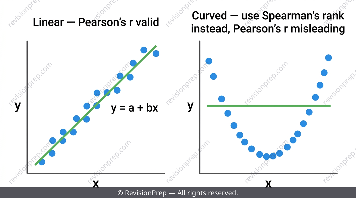
Pearson's $r$ measures only LINEAR association — feed it a curved (monotonic-but-bending, U-shaped or hump-shaped) scatter and you'll get a misleadingly small value that does NOT mean 'no relationship'. For monotonic curved data, switch to Spearman's rank $r_{s}$ ; for genuinely non-linear shapes, consider a non-linear regression model instead. Once you fit $y = a + b x$ , predicting within the observed x-range is fine — predicting far outside it is extrapolation and must be flagged as unreliable.

Two scatter plots side by side: one linear with a regression line, one curved (U-shaped) with a note that Pearson's r is misleading

Exam tip

Look at the scatter shape BEFORE calculating anything: only calculate Pearson's r if the pattern looks straight-line-ish.

Common mistake

Plugging an x-value far outside the data range into a regression equation and reporting the result as a reliable prediction without commenting on extrapolation.

Mini summary

r = linear fit only; check the shape first, and always flag extrapolation explicitly.

Unbiased Estimators and Confidence Intervals

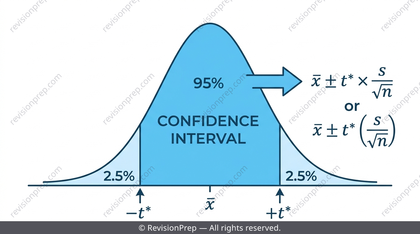
An unbiased estimator's expected value equals the true population parameter — $\overset{x}{ˉ}$ is an unbiased estimator of $μ$ . A confidence interval is a range of plausible values for $μ$ built around $\overset{x}{ˉ}$ ; a 95% CI means that if you repeated the sampling process indefinitely, 95% of such intervals would capture the true $μ$ — it does NOT mean there's a 95% chance $μ$ lies in this particular interval. At HL, $σ$ is almost always unknown, so you use the t-distribution with $n - 1$ degrees of freedom, not z.

Bell curve with 95% confidence interval shaded around the sample mean x-bar, with t-distribution critical values marked

Exam tip

Before reaching for a critical value, ask: is σ actually given, or only s? That single check decides between z and t.

Common mistake

Using $z = 1.645$ instead of $t_{n - 1}$ just because the sample size 'feels big enough' — the choice depends on whether σ is known, not on n.

Mini summary

CI = range for the parameter; use t (not z) whenever only sample s is known — which is almost always at HL.

Hypothesis Testing: z, t and Paired t-Tests

A hypothesis test assumes $H_{0}$ is true, checks how surprising your sample result would be under that assumption (the p-value), and rejects $H_{0}$ only if p is below the significance level. Use a z-test when σ is given, a one-sample t-test when only s is known, and a paired t-test when comparing matched before/after differences $d_{i}$ for the same subjects.

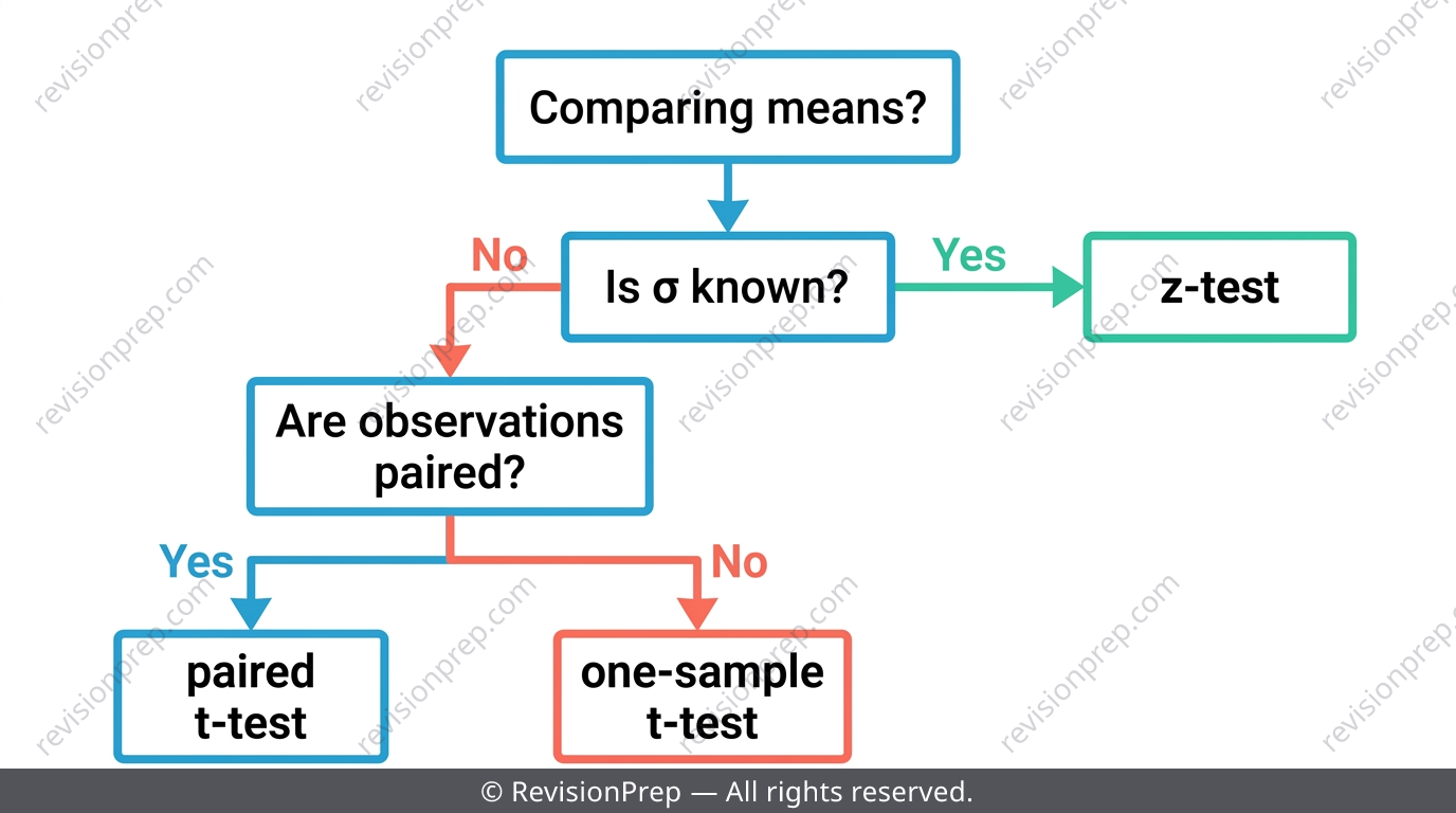
Flowchart deciding between z-test, one-sample t-test and paired t-test based on whether sigma is known and whether data is paired

Scenario	Test	Key formula
σ known, one sample	z-test	z = (x̄ − μ₀)/(σ/√n)
σ unknown, one sample	t-test	t = (x̄ − μ₀)/(s/√n), df = n−1
Matched before/after pairs	Paired t-test	t = (d̄ − μ₀)/(s_d/√n), df = n−1

Exam tip

Every hypothesis test answer needs four visible parts: hypotheses in symbols, test statistic/p-value, comparison to α, and a conclusion written IN CONTEXT.

Common mistake

Stopping at 'z = -1.77, so reject H₀' without the final sentence explaining what that means in context — that sentence carries its own separate mark.

Mini summary

Check σ known vs unknown to pick z or t, and never skip the in-context conclusion sentence.

Chi-Squared Tests for Independence

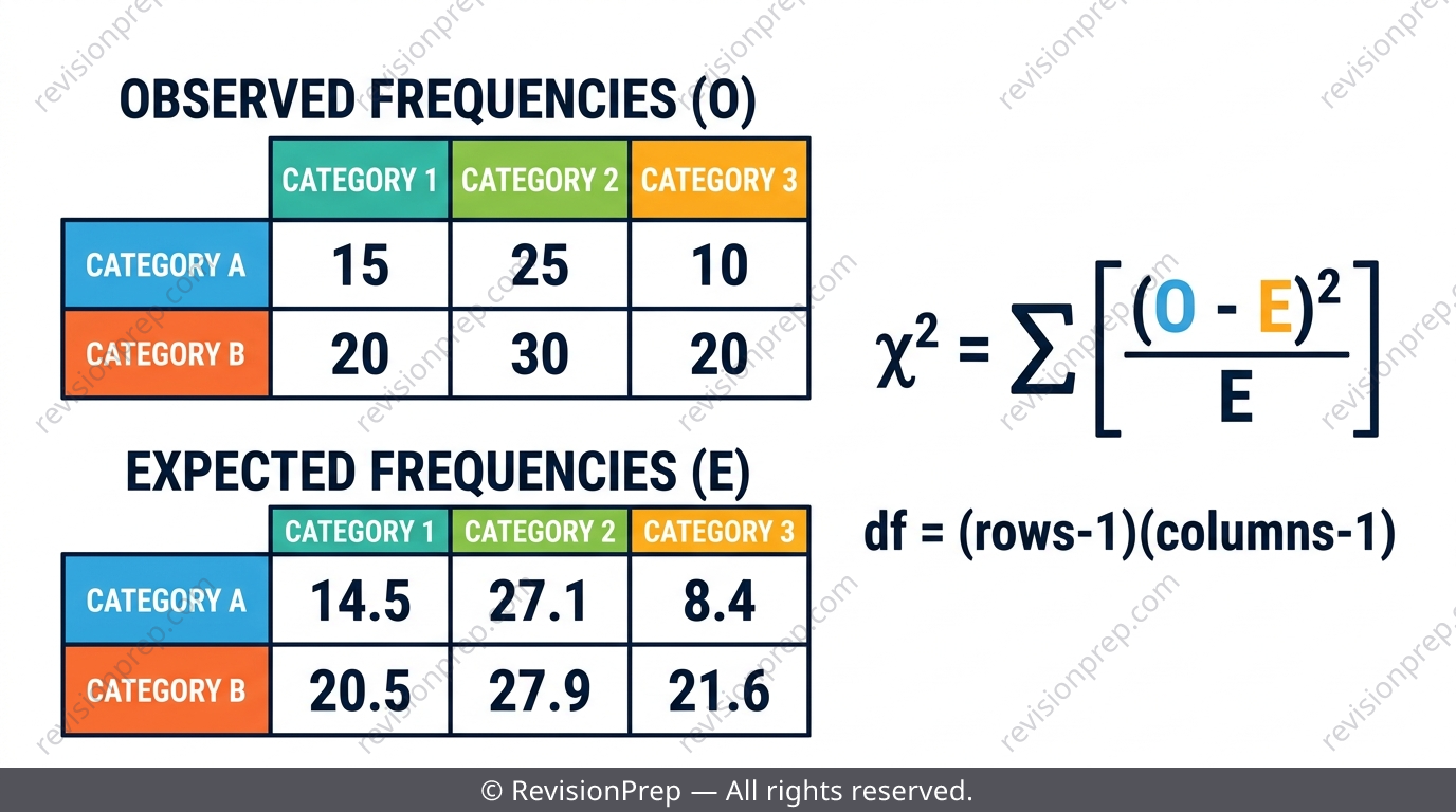
The chi-squared test compares observed frequencies $O$ against expected frequencies $E$ (calculated assuming independence) using $χ^{2} = \sum \frac{( O - E ) ^{2}}{E}$ , with degrees of freedom $(rows - 1) (columns - 1)$ . Expected frequencies should generally be at least 5 for the test to be valid, and getting df wrong is one of the most common ways to lose marks even when the χ² arithmetic is perfect.

A 2x3 contingency table showing observed and expected frequencies with the chi-squared formula and degrees of freedom calculation beside it

Exam tip

Write 'df = (rows−1)(columns−1) = ...' as its own labelled line before touching the critical value table or GDC p-value function.

Common mistake

Using n−1 or rows×columns instead of (rows−1)(columns−1) for degrees of freedom — a perfectly calculated χ² value with the wrong df row loses the final marks.

Mini summary

Same χ² formula for independence and goodness-of-fit; always state df explicitly and check E ≥ 5.

Quick formula sheet

\overset{x}{ˉ} \pm t_{n - 1} \cdot \frac{s}{n}

Confidence interval for μ when σ is unknown (almost always at HL) — s unknown → use t, not z

z = \frac{x ˉ - μ _{0}}{σ / n}

One-sample z-test statistic, only when σ is given — z needs σ (Greek letter, given value)

t = \frac{x ˉ - μ _{0}}{s / n}, df = n - 1

One-sample t-test statistic when only sample s is known — t for 'to be estimated' — df is always n−1

t = \frac{d ˉ - μ _{0}}{s _{d} / n}, df = n - 1

Paired t-test on the differences d between matched observations

s_{n - 1}^{2} = \frac{n}{n - 1} σ_{n}^{2}

Unbiased estimate of the population variance from a sample — n−1 corrects the under-estimate from dividing by n

E = \frac{( row total ) \times ( column total )}{grand total}

Expected frequency in a contingency table cell under independence

χ^{2} = \sum \frac{( O - E ) ^{2}}{E}

Chi-squared test statistic, same formula for independence and goodness-of-fit

df = (rows - 1) (columns - 1)

Degrees of freedom for a chi-squared test of independence

r = \frac{S _{x y}}{S _{xx} S _{y y}}

Pearson's product-moment correlation coefficient (linear association only)

b = \frac{S _{x y}}{S _{xx}}, a = \overset{y}{ˉ} - b \overset{x}{ˉ}

Least-squares regression line y = a + bx (y on x)

Practice questions

Easy

State the difference between simple random sampling and stratified sampling.
A sample of size 15 gives σₙ = 2.1. Find the unbiased estimate s₍n-1₎².
Write down the null and alternative hypotheses for testing whether a population mean has increased from 50.

Medium

A sample of 12 items gives x̄ = 8.42 and s = 0.35. Construct a 90% confidence interval for μ, stating which distribution you use and why.
For a 2×3 contingency table with row totals 80, 50 and column totals 60, 40, 30 (grand total 130), find the expected frequency for the cell in row 1, column 2.
Explain why using Pearson's r on data with a clear U-shaped scatter would be misleading, and state an alternative measure.

Challenge

Differences (after − before) for 8 students are 3, 5, −1, 7, 2, 4, 6, 2. Test at the 5% level whether the new method improves scores, stating hypotheses, test statistic and a conclusion in context.
A χ² test of independence on a 2×3 table gives χ² ≈ 7.72. Determine the degrees of freedom, compare to the critical value at the 5% level, and write a conclusion in context.
A regression line is fitted to age (0–10 years) and length data for fish. Explain why using this line to predict length at age 50 would be inappropriate, and describe what should be stated instead.

Frequently asked questions

What's the difference between a confidence interval and a hypothesis test?+

A confidence interval gives a range of plausible values for the population parameter itself, while a hypothesis test checks whether one specific claimed value is plausible given the sample. Both use the same t or z machinery, but they answer different questions.

When do I use a z-test instead of a t-test in IB Maths AI?+

Use a z-test only when the population standard deviation σ is explicitly given. If you only have the sample standard deviation s, use a t-test with df = n − 1, regardless of how large the sample is.

Why is sample variance divided by n−1 instead of n?+

Dividing by n underestimates the true population variance on average. Dividing by n−1 corrects this bias, giving the unbiased estimate s²ₙ₋₁ that your GDC labels separately from σₙ².

How do I find degrees of freedom for a chi-squared test?+

For a test of independence, df = (rows − 1) × (columns − 1). Writing this as its own labelled line before using a critical value table or GDC avoids one of the most common exam errors.

Why can't I use Pearson's r for curved data?+

Pearson's r only detects linear association. A curved scatter (monotonic or U-shaped) can produce a small r even when there's a strong relationship — use Spearman's rank correlation or a non-linear regression model instead.

What does a 95% confidence interval actually mean?+

It means that if you repeated the sampling process many times, about 95% of the resulting intervals would contain the true population mean. It does not mean there's a 95% probability the mean lies in this one specific interval.

Get the full Statistics and Probability revision notes

Step-by-step worked examples for every confidence interval and hypothesis test type Full explanations of χ² independence and goodness-of-fit tests with GDC steps Mock papers and exam-style questions with detailed model answers Printable formula sheet covering the entire IB DP Maths AI statistics syllabus

Get the Statistics and Probability notes on RevisionPrep →

Maths AI: Geometry and Trigonometry (SL)Maths AI: Geometry and Trigonometry (HL)Maths AI: Statistics and Probability — Correlation & Chi-Squared